In this example we show the results of various methods that can be used to determine the misfit between different shear wave splitting (SWS) parameters and illustrate how these can be used to fit a model to measured SWS data. The four methods that are implemented in MSAT which can be used to estimate the difference between one splitting parameter, $\Gamma_1 = (dt_1 , \phi_1)$, and a second, $\Gamma_2 = (dt_2 , \phi_2)$, are first outlined and results illustrated. In the second part of the example we show how this approach can be used to find the best-fitting model assuming tilted transverse isotropy (TTI) to a collection of synthetic SWS measurements.
Calculating a misfit
The example file demo_splitting_misfit.m in the examples/splitting_misfit
directory shows how the MSAT function MS_splitting_misfit can be used
and plots the value of the misfit function for pairs of splitting
parameters. The reference splitting parameters, $\Gamma_1$,
for this illustration are $dt_1 = 2$ seconds and
$\phi_1 = 0$ degrees. This is compared with
$\Gamma_2$ with values varying from
$\phi_2 = -90$ to $\phi_2 = 90$ degrees and
$dt_2 = 0$ to $dt_2 = 4$ seconds. For the methods
that are sensitive to source polarization three values are used, 45,
30 and 0 degrees. The calculation of misfit over this grid of values
of $\Gamma_2$ is done as follows in the function
calc_misfit_surface:
   fast = [-90:5:90] ;
   tlag = [0:0.1:4] ;

   [TLAG,FAST] = meshgrid(tlag,fast) ;
   MISFIT = FAST.*0 ;

   % generate misfit
   for itlag=1:length(tlag)
      for ifast=1:length(fast)
        MISFIT(ifast,itlag) = ...
           MS_splitting_misfit(fast_ref,tlag_ref, ...
              fast(ifast),tlag(itlag),spol,0.1,'mode',modeStr,'max_tlag',10) ;
      end
   end
The call to MS_splitting_misfit calculates the misfit for each of the
values of $\Gamma_2$. This is done for each of the
polarisation directions and misfit calculation methods ("simple",
"intensity", "lam2" and "lam2S") and the calculated misfit
surfaces plotted.
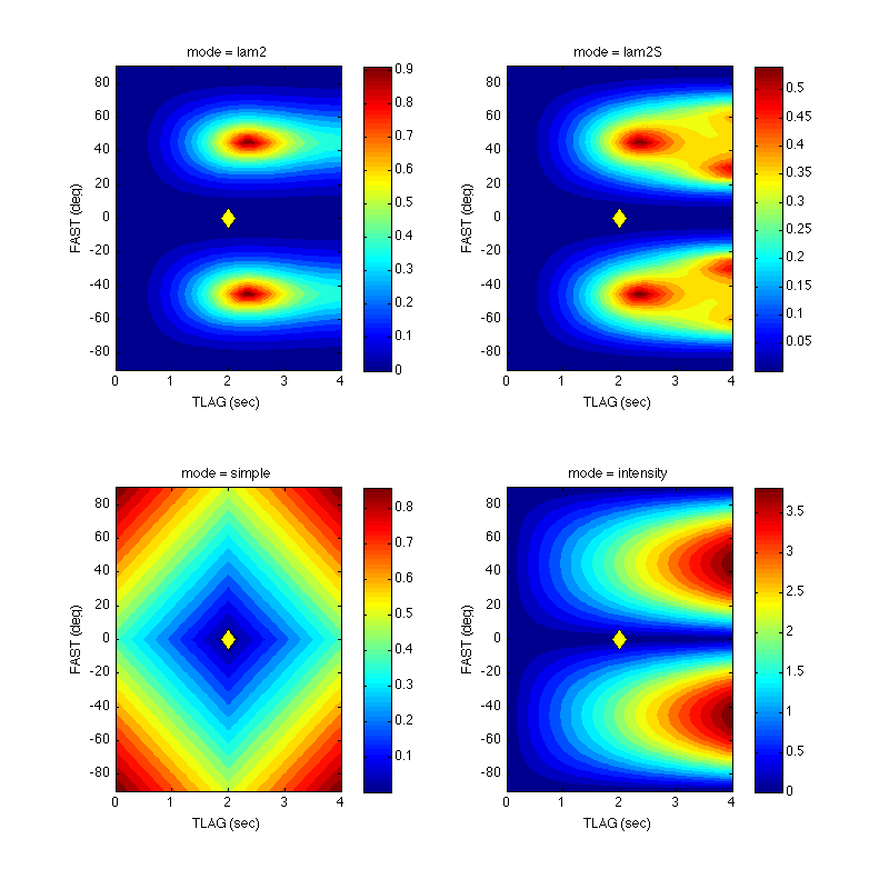
The images above show the misfit surfaces produced by the
demo_splitting_misfit example for the 0 degree polarisation angle.
It is instructive to first consider the "simple" approach (lower left
figure). This approach takes the average of the magnitude of the
difference between the delay times and magnitude of the difference
of between the fast directions. That is:
$\displaystyle{\frac{1}{2} \left(\frac{|dt_1-dt_2|}{(0.25/f_d)} + \frac{|\phi_1 - \phi_2|}{90}\right)}$,
where $f_d$, the dominant frequency, and 90 are included to properly normalise the two parts of the sum. This is not dependent on the initial polarisation direction and always forms a diamond shape with a minimum located at the point where $dt_1 = dt_2$ and $\phi_1 = \phi_2$. Another approach is the comparison of splitting intensity activated by the "intensity" method. The approach is to calculate the splitting intensity for both pairs of parameters:
$\displaystyle{S_i = dt_i \sin(2 \beta_i)}$,
(where $\beta$ is the difference between the initial polarisation angle and $\phi$) and taking the magnitude of the difference between $S_1$ and $S_2$. As shown in the lower right figure, the misfit surface is more complex but retains a minimum where the two splitting operators are equal. MSAT also implements two other approaches motivated by the way that SWS parameters can be extracted from data and, in particular the minimum eigenvalue method (Silver and Chan, 1991). Details of the approach, which involves splitting a probe wavelet using $\Gamma_1$, "unsplitting" it using $\Gamma_2$, and comparing the result with the probe wavelet, is given in the user guide but the result is shown in the top two figures. The top left figure shows the results of the "lam2" method which, because SWS operators are not commutative, differs if the values of $\Gamma_1$ and $\Gamma_2$ are exchanged. The top right figure shows the "lam2S" method where the forward and reversed "lam2" results are averaged to give a misfit function which is independent of the order that the splitting functions are supplied. The misfit function for both eigenvalue based methods change with both the initial polarisation angle and the dominant frequency of the test wavelet. In the following section the "lam2" misfit function is used to derive and elastic model that best fits SWS results.
From a misfit to a model
The file examples/splitting_misfit/fit_TTI_orientation.m shows how the splitting
misfit described above can be used to find an elastic model that matches a set
of SWS measurements. In the following example an elastic model with tilted
transverse anisotropy (TTI) is generated and used to calculate three splitting parameters
that would correspond to observations of rays arriving from different azimuths and
inclinations. A grid search over different orientations of the TTI medium is then
performed and at each orientation the model’s predicted splitting parameters are
calculated. These are then compared with the "observations" and the orientation that
minimises the sum of the misfit found. This orientation is then reported (along with
the resulting misfit surface. Key parts of the code for this example are
described below
The first step is to generate an elasticity matrix describing the "observed" TTI medium and calculate the "observed" splitting parameters. The model is set up as follows:
   %% set the raypath parameters. ---------------------------------------------
   razi = [045 135 048] ;
   rinc = [000 000 032] ;
   dist = 50 ; % km

   %% set up the medium to be modelled. ---------------------------------------
   str = 60 ;
   dip = 25 ;

   vpi=2;
   vsi=1;
   rh=2000;

   [Craw]=MS_VTI(vpi,vsi,rh,0.05,0.05,0.05) ;
and we note that (as is commonly the case for SWS) there is no way to distinguish
a thin layer of strong anisotropy from a thick layer of weak anisotropy. We thus
assume a 50 km thick layer of fixed strength of anisotropy throughout and only solve
for the orientation of this layer. The "observed" parameters are returned by a
the function call [fast,tlag,ravs]=create_dataset(Craw,rh,str,dip,razi,rinc,dist) ;,
which makes use of MS_phasevels.
The second stage of the calculation is to compute the misfit between fast and
tlag and the calculated splitting parameters for a range of TTI orientations.
This is done in the loop over strikes and dips thus:
   %% calculate a grid of misfits over a range of strikes and dips. -----------
   fprintf('Grid searching over strike and dip ... \n')
   [GSTR GDIP] = meshgrid([0:10:360],[0:5:90]) ;
   GMIS=GSTR.*0 ;
   [n,m]=size(GSTR) ;
   for i=1:n
      for j=1:m
         str_dip = [GSTR(i,j) GDIP(i,j)] ;
         GMIS(i,j) = orientation_misfit(str_dip,Craw,rh,...
            0,0.1,fast,tlag,razi,rinc,dist) ;
      end
   end
with the misfit stored in GMIS. Calculation of the misfit for each orientation
is performed by the orientation_misfit function with the body of the calculation
involving the use of MS_phasevels and MS_splitting_misfit for each "observed"
splitting function:
% rotate the test matrix
[Ctest]=MS_rot3(Cbase,0,-str_dip(2),str_dip(1)) ;
% calculate associated splitting
[pol,avs,vs1,vs2,~,~,~] = MS_phasevels(Ctest,rh,rinc,razi) ;
fast = pol ;
tlag = dist./vs2 - dist./vs1 ;
% calculate the misfit (the average over all raypaths)
misfit=0 ;
for i=1:length(data_fast)
misfit = misfit + MS_splitting_misfit(data_fast(i),data_tlag(i),...
fast(i),tlag(i),data_spol,data_dfreq,'mode','lam2') ;
end
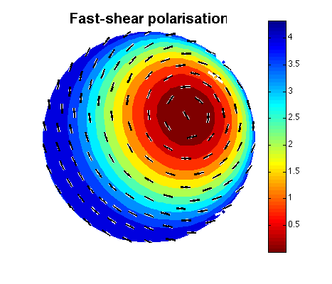
misfit = misfit ./ length(data_fast) ;The final step is to report and plot the best fitting model and misfit surface. The
model and "observations" are plotted together using the "sdata" option in MS_plot:
   fprintf('Plotting model and observations\n')
   Cbest = MS_rot3(Craw, 0, -GDIP(imin,jmin), GSTR(imin,jmin));
   MS_plot(Cbest,rh,'sdata',razi,rinc,fast',ravs','plotmap', {'avspol'}) ;
which produces the diagnostic pole figure below. In this figure "observed" SWS data (white lines, coloured spots refer to strength of anisotropy) and the best fitting model (black lines, coloured contours refer to strength of anisotropy) are both shown.