It is often necessary to interpolate elastic constant tensors
between values at known points. Naive element-by-element
interpolation can result in anomalous seismic velocities. MSAT
includes an interpolation technique involving both the
orientation (defined in terms of the eigenvectors of the
Voigt stiffness tensor) and magnitude of the two end-member
elastic tensors. This approach is available using MS_interpolate.
Element-by-element interpolation can be performed using MS_VRH.
This example is a comparison of the two approaches.
|
Note
|
Method
The interpolation method used in
|
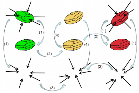
The example interpolates between two end-member elasticities, which are read from the MSAT database and rotated in different directions:
% Forsterite: X = 0
[C_x0, rh_x0] = MS_elasticDB('olivine');
C_x0 = MS_rot3(C_x0, 0, 0, 60);
% Fayalite: X = 1
[C_x1, rh_x1] = MS_elasticDB('fayalite');
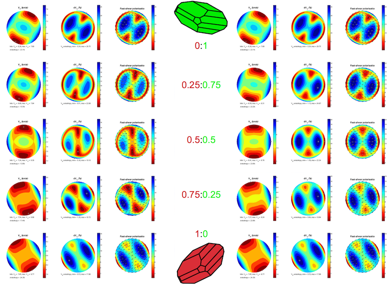
C_x1 = MS_rot3(C_x1, 0, 0, 120);Interpolation is then done in a loop changing the fraction of forsterite and fayalite in 400 steps between the two end members. Five values (0.0:1.0, 0.25:0.75, 0.5:0.5, 0.75:0.25 and 1.0:0.0) are selected for plotting. The key code to undertake element-by-element (Voigt) interpolation is:
[~, rh_interp, C_voigt] = MS_VRH([x 1-x], C_x0, rh_x0, C_x1, rh_x1);The MS_interpolate function works in a similar way:
[C_interp, rh_interp] = MS_interpolate(C_x0, rh_x0, C_x1, rh_x1, x);Comparison of methods
element-by-element (Voigt) and our symmetry preserving interpolation methods are compared in the figure below for the case of interpolation between forsterite and fayalite with different crystallographic orientations. Element-by-element (MS_VRH) interpolation smears out the phase velocity surface and introduces low symmetry components, while the MS_interpolate approach maintains orthorhombic symmetry throughout.
Performance
MS_interpolate takes about 20 times longer to find the interpolated
elasticity than MS_VRH. Timing analysis can be performed using the
"calc_times" argument to the example:
>> interpolate_1D_example('calc_times')
Time per Voigt interpolation = 0.000109 s
Time per common orientation interpolation = 0.001872 s