MSAT quick start guide.
Installation
Installation of the MATLAB toolbox is described here.
Seismic anisotropy in MSAT
Seismic anisotropy - the variation of seismic wavespeed with direction, is a fundamental property of most solid Earth materials. This variation is encapsulated in the elasticity tensor C (sometimes called the stiffness), which describes the relationship between stress and strain in a material:
$\sigma_{ij} = C_{ijkl}\epsilon_{kl}$
This is, in general, a 4th rank tensor (3x3x3x3). However, it can be represented as a more convenient symmetric 6x6 matrix (usually called Voigt notation) with no loss of information. This 6x6 notation is the default used by MSAT (though utilities for conversion to and from the 4th rank form are provided). The 6x6 C matrix (along with the density for some functions) are the main data used in MSAT, which provides functionality to load, manipulate, analyse and plot elasticities.
Default units
We adopt unit conventions which should be familiar to most people conversant with the current literature:
| Quantity | Unit |
|---|---|
Elasticity |
gigapascals |
Density |
kg/m3 |
Velocity |
km/s |
Option exist to import elasticities in other units, however (see MS_load for details).
Loading elastic constants.
Elastic constants can be sourced from MSATs own built-in database (see MS_elasticDB for details) which contains a number of useful minerals, or from an ascii file. The available formats of the files are given in the documentation to MS_load, and examples are available in the msat/examples/loading.
To get elastic constants for olivine (from REF) for example:
>> [C,rho] = MS_elasticDB('Olivine')returns
C =

  320.5000   68.1000   71.6000         0         0         0
   68.1000  196.5000   76.8000         0         0         0
   71.6000   76.8000  233.5000         0         0         0
         0         0         0   64.0000         0         0
         0         0         0         0   77.0000         0
         0         0         0         0         0   78.7000


rho =

        3355
Manipulating elastic constants
Once the stiffness matrix (and density) are laoded MSAT provides a set of routines for performing various manipulations and transforms of them (see the user guide for full list). For example, the function MS_rot3 applies rotations about the principle cartesian axes to an elastic tensor. So, for example:
>> C = MS_elasticDB('Olivine')

C =

  320.5000   68.1000   71.6000         0         0         0
   68.1000  196.5000   76.8000         0         0         0
   71.6000   76.8000  233.5000         0         0         0
         0         0         0   64.0000         0         0
         0         0         0         0   77.0000         0
         0         0         0         0         0   78.7000

>> CR = MS_rot3(C,90,0,0)
returns
CR =

  320.5000   71.6000   68.1000    0.0000         0         0
   71.6000  233.5000   76.8000    0.0000         0         0
   68.1000   76.8000  196.5000    0.0000         0         0
    0.0000    0.0000    0.0000   64.0000         0         0
         0         0         0         0   78.7000   -0.0000
         0         0         0         0   -0.0000   77.0000
which is the expected orientation of horizontally-strained olivine under dry upper mantle conditions.
Analysis
As well as transformations, MSAT provides routines for analysing various aspects of stiffness tensors. For example, MS_anisotropy calculates a variety of simple measures of the anisotropy of an input elastic tensor:
>> C = MS_elasticDB('Albite') ;
>> uA = MS_anisotropy(C)

uA =

    2.0694
where uA is the Universal Elastic Anisotropy Index of Ranganathan and Ostoja-Starzewski (2008).
Visualisation
Finally, MSAT can be used to create various kinds of visualisations of elasticity matrices. For example:
>> [C,rh] = MS_elasticDB('Albite') ;
>> MS_sphere(C,rh,'S')
produces:
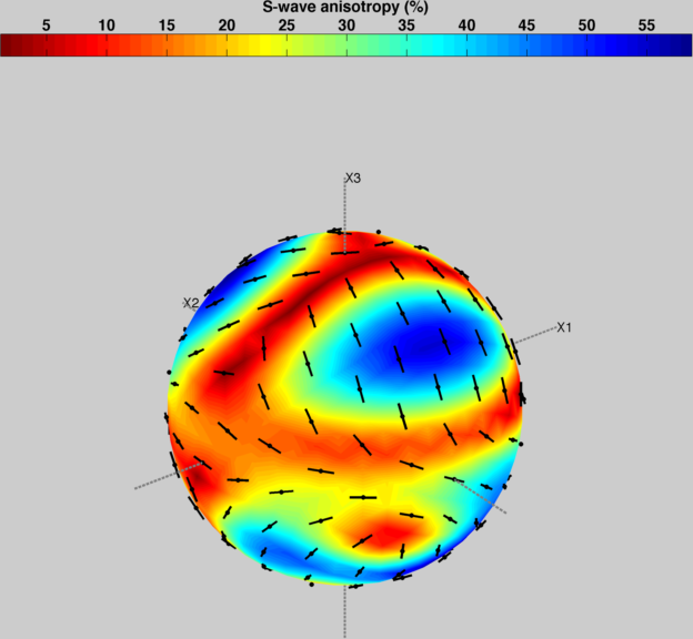
which shows the variation of shear-wave anisotropy (and fast-shear wave orientation) for single crystal albite.
More help
A more in-depth guide to MSAT is provided by the user guide. Further information (upgrades, reporting bugs, how to install) can be found at the MSAT website (http://www1.gly.bris.ac.uk/msat). There is also a paper published in Computers and Geosciences (volume 49, pages 81 - 90) describing MSAT. This is available online as a preprint or from Elsevier.